
xG stands for Expected Goals. xG is – as of this writing (4-10-2019) the hottest stat for football. xG basically calculates for a discrete number of positions the ratio of how many times a player has scored from that position and how many times players have shot from that position. Using Frequentism, people than equate xG with the chance to score from that position. This is only correct from the standpoint of Frequentism. If your frame of reference is Bayesian statistics then the frequency of scoring from a certain position is one of many things you can weigh in your judgement what the chance is for a particular player to score from that position against that particular opponent in that particular game. The lack of context is one of the criticisms that have been leveled against xG.
The following thought experiment demonstrates the importance of context. Say spot X has an xG of 0.5, meaning that 50% of shots taken from that position score a goal. If we found out that there were two evenly divided groups of players: group A and group B. If we then learn that players in group A always miss when shooting from spot X and that players in group B always score. Then we know exactly why spot X has an xG of 0.5. But it also makes clear that when a random player is shooting from spot X, there is much more value in knowing whether he belongs to group A or group B, then knowing the xG value of spot X. If you know the player is in group A, then you know he is going to miss. If you know the player is in group B, then you know he is going to score. The problem is that we don’t know whether a player is in group A or group B. We don’t even know which groups exist. xG is a way to compensate for this information. But football statistics would be a lot better if we were able to discern these groups and know which players belong to which group. In this way you can add more contextual information like the strength of the opposing team, time passed in the match or fatigue, for instance.
Nevertheless, the use of xG has been argued for by referring to the idea that xG has the highest correlations with other backward and forward looking statistics. First of all this is not the case. It is already known that the correlation of xG really only works in the top four leagues. For instance, in the Scottish football, shots on goal was a better stat to determine the winner than xG. My own research looking at the center forward of the clubs in the Dutch Eredivisie and the Belgium Jupiler Pro League only gave a 27% correlation with goals in the next season versus our own proprietary median FBM Attack score having a 50% correlation with future goals.
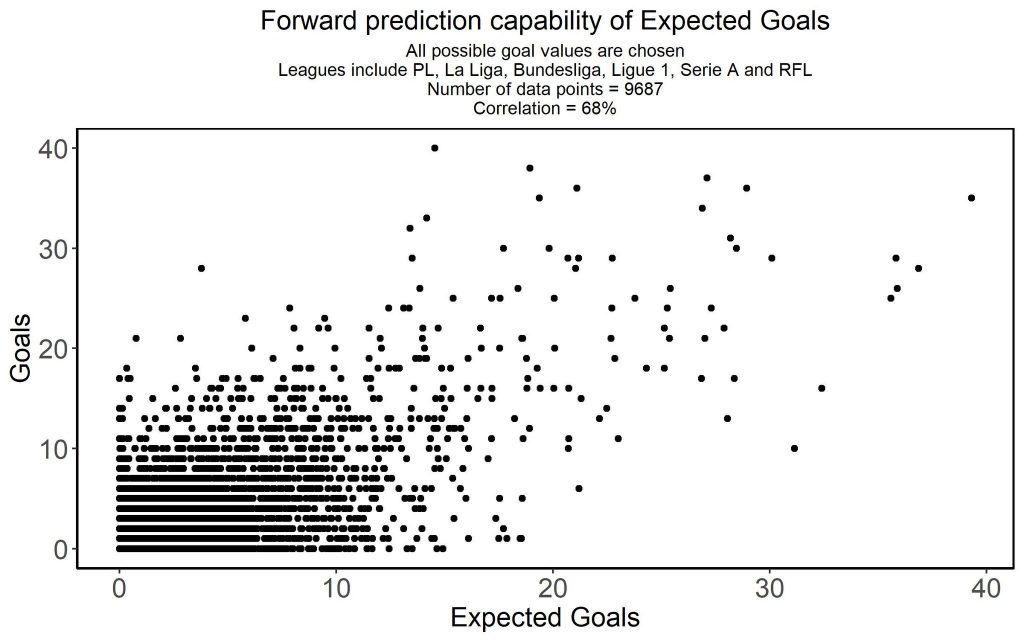
Since then quite a few people have calculated the correlation of xG and future goals in a number of different scenarios. Personally I am grateful to Ashes on Twitter for calculating different sets of correlations. Most people find that xG has a 68% correlation with the number of goals scored in the next season. Yet, there are many issues with correlation that make this number look more impressive than it really is as Ashes has been so kind as to help me demonstrate.
What is wrong with correlation and xG
The easiest problem with correlation is that any correlation below 80% carries very little information. Here are six diagrams showing you how much information there is, given a certain level of correlation:
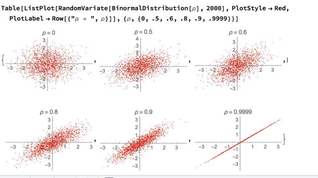
As you can see a correlation as high as 60% still carries very little information. That is the reason that although we found that our proprietary median FBM Attack score has a 50% correlation with future goals scored by the center forward of Belgian and Dutch clubs, we don’t use that to scout players as it would fool us. Yet, you can also see that a 27% correlation is also completely useless. So although there is a bit more information in a 68% correlation, the fact that it is below 80% makes it useless for decision making.
But the 68% correlation is misleading. Again, thanks to the work of Ashes, you can see that the 68% correlation is artificially inflated by combining the high correlation of low performing players, with the low correlation of high performing players. This issue has been discovered by Nassim Taleb in his criticism of IQ. What I have done with the help of Ashes, is apply the same principle to xG. Here are the results:
In the next chart Ashes only looks at players who have at least scored five goals:
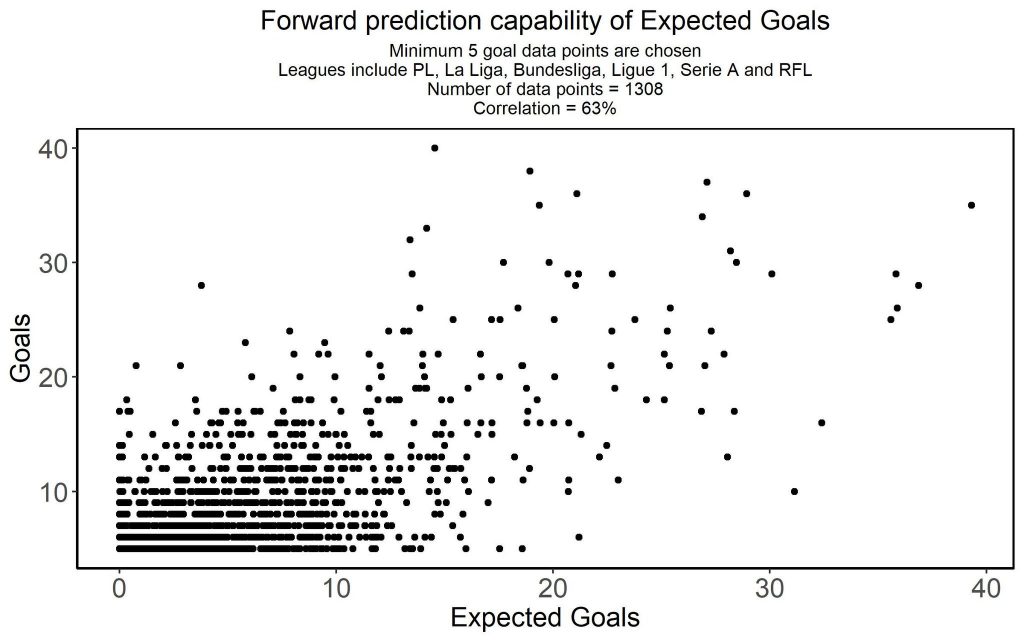
As you can see now that we are excluding the worst performing players in regards to scoring, the correlation drops from 68% to 63%. This trend continues the more low performing players we eliminate:

With at least 10 goals scored, the correlation drops to 58%.
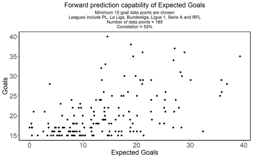
And with at least 15 goals scored the correlation drops to 53%. Now take a look again at the graphs that show how little information there is for a 50% correlation:
Here is a graph that makes it even more clear how the correlation with future goals decreases the better the player is:

Also xG overperformance has a low correlation with future xG:

So selecting players based on their current overperformance on xG stat is a bad strategy. If you look at future goals there is no correlation:

xG in the Eredivisie
To remind you: Ashes has looked at the top 5 leagues and the Russian league. Personally, I am more interested in the smaller leagues, especially the Eredivisie. And I am more interested in whether it helps to use xG in concrete player recruitment, especially in finding exceptional players. At my work at FBM we have found the striker Dalmau for Heracles. Not only did Dalmau become the #3 top scorer that season, we also predicted that he would be worth 1.75 million in transfer fee for Heracles the next year and Heracles did receive 1.7 million for Dalmau (700K transfer fee and Dessers, a striker valued at 1 million).
So in order to see how xG correlates with goals in the next season, I looked at three very specific groups within the top 100 top scorers for the 18/19 season and calculated the correlations with xG (and some other stats to compare) from the 17/18 season. For the top 100 the result is a correlation of 48%. As correlation is nothing more than a measure of how much two lines look the same, it helps to actually look at the graph of the data:
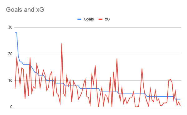
As you can see even though the correlation is 48%, in reality there is very little information in this graph. A lot of the correlation found has to do with the fact that the goals scored is a very nice, well behaved line, which is logical given that the line is ordered by goals scored.
But things get even more interesting when we look at the top 30 rather than the top 100. Now the correlation of xG with goals in the next season drops to as little as 20%! Which you could already have seen in the previous chart, but becomes painfully obvious in the next chart:
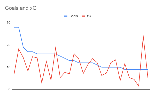
As you can see there is no information to be found in this chart.
In fact for the top 30, minutes played has a 37% correlation with goals scored the next season. To be clear, that is still way less than you need for decision making, but it puts to bed the idea that if you want top scoring players, you should look at xG. In fact our proprietary stat scores a 53% correlation for the top 30 top scorers of the Eredivisie, but again this is not enough for decision making.
Here is the table of the different stats I look at for the top 30, top 60 and top 100:
| xG/90 | xG | SOT/90 | SOT | Minutes | Goals scored in season | |
| Top 30 | 7.43% | 19.45% | 1.47% | 17.23% | 36.66% | 13.92% |
| Top 60 | 28.45% | 36.68% | 30.78% | 33.33% | 30.61% | 23.68% |
| Top 100 | 39.90% | 47.99% | 37.36% | 45.34% | 30.09% | 40.52% |
As you can see it really makes little difference whether you look at xG or at Shots On Target (SOT). This further backs up the data found in the Scottish competition. From spot #62 on players have scored 5 or less goals in the Eredivisie. As you can see by adding low performing but highly correlated players to the population, you increase the correlation.
Now one criticism might be that the top 30 is too small. Although 30 sounds like a small sample size, 30 is often used as the minimal sample size. Sample size ought to reflect what we are looking for. When it comes to using xG for the recruitment of players, what clubs are looking for are players who can make a difference scoring wise. Preferably, clubs hire players who score a lot, but cost a little. Dalmau moved to Heracles transfer free. Clubs want players who score above average. Or in other words: clubs are looking for players who make it to the top 30! If they use xG to base their decision making on, they are going to make too many bad decisions.
Circularity
Yet, the story of xG and correlation becomes even worse. For we haven’t taken circularity into account. If you look at the formula for xG, all data providers have different ways of calculating xG. Nevertheless, it basically is:
xG = goals scored by shooting from position X / total shots from position X
If you look at the correlation between xG and goals, one needs to account for the circularity of it all. For goals are part of the formula in xG. Having the thing you calculate your correlations for as part of the formula you use to determine the correlate in the first place, creates circularity. Circularity means that the correlation will be a bit higher than it would have been without circularity. So all the above correlation for xG and goals scored the next season are overestimations due to circularity!
[Update 21-11-2022: I found out that there is no correlation between goals and xG. This is of course not a criticism as xG and goals aren’t meant to correlate as xG is an alternative way of trying to explain the match other than the actual goals. Nevertheless, it is note worthy that this means that xG has zero explanatory power in explaining goals. To be clear: a high correlation between xG and goals would actually be bad for xG as xG is an alternative measure to explain the match than goals. If the correlation were to be high, it wouldn’t be an alternative.]
A bad map is better than no map at all
The final defense of xG by its proponents, is that xG might not have correlation that are high enough to give you useful information, but at least it is the best we can do. First of all, this is simply not the case. There are a number of examples, for instance the Scottisch Premier League, where Shots On Target did better. But even if it were the case, then it is still a fallacy.
This fallacy is called the “bad map is better than no map at all” fallacy. This is a fallacy because logically, you have a better chance of finding the correct way without a map, than with a bad map. A simple thought experiment we philosophers like so much, will demonstrate this.
Imagine you are in a maze and you have four different paths to go: north, east, south, west and two people. Person A without a map and person B with a bad map, even though he thinks, incorrectly, that he has a good map. If that is all we know, most people would give person A a chance of 25% of choosing the right path. But as it is highly likely that person B will choose the path that his map incorrectly highlights as the correct path. So the chance of person B actually choosing the right path is probably below 1%. Such is the danger of incorrect maps!
The solution
After describing so much of what is wrong with using xG for player recruitment, let me also explain a healthy alternative. Rather than using a single stat, one builds a Bayesian network that includes all sources at the club. Sources included all independent data sources, scouts, coaches, the manager, head of recruitment, technical director and the finance guys. Based on their inputs the Bayesian network calculates for all players in the shadow team what the probability is that player X is able to contribute to the team. And preferably also calculates how much money a club can probably make with a future transfer fee. Then the Bayesian network automatically orders all players in the shadow team to come up with the most rational decision when it comes to recruiting the right player.
PSxG
[Update 30-7-2020] What a difference nine months can make! The original post was written in october 2019. Since then xG has been uprooted by PSxG or Post Shot xG, also known as xG Shots on Target. As it turns out taking looking primarily only at the shots that were actually on the target, i.e. shots that either scored or would have scored if no opponent would have interfered, we get a more informative stat.
This can for example be seen in the Premier League at the difference between xPoints based on xG and xPoints based on PSxG. xPoints are expected points scored in the league based on either xG or PSxG.
For xG it looks like this (table courtesy of https://twitter.com/ParthAthale) :
| Rank | Points | xPoints based xG | |
| Liverpool | 1 | 99 | 74 |
| ManCity | 2 | 81 | 87 |
| ManUnited | 3 | 66 | 71 |
| Chelsea | 4 | 66 | 73 |
| Leicester | 5 | 62 | 61 |
| Tottenham | 6 | 59 | 49 |
| Wolves | 7 | 59 | 63 |
| Sheffield | 7 | 54 | 49 |
| Arsenal | 8 | 56 | 50 |
| Burnley | 10 | 54 | 49 |
| Southampton | 11 | 52 | 57 |
| Everton | 12 | 49 | 55 |
| Newcastle | 13 | 44 | 31 |
| Crystal | 14 | 43 | 38 |
| Brighton | 15 | 41 | 47 |
| West Ham | 16 | 39 | 38 |
| Aston Villa | 17 | 35 | 37 |
| Bournemouth | 18 | 34 | 39 |
| Watford | 19 | 34 | 47 |
| Norwich | 20 | 21 | 31 |
The correlation between rank is 84% and with points is 73%. The 84% correlation is above 80% so that is a decent correlation, but unfortunately for points the correlation is below 80% and hence not really informative.
If we do the same with PSxG rather than xG, we get (courtesey of https://twitter.com/StatifiedF ):
| Rank | Points | xPoints based on PSxG | |
| Liverpool | 1 | 99 | 89 |
| ManCity | 2 | 81 | 81 |
| ManUnited | 3 | 66 | 69 |
| Chelsea | 4 | 66 | 68 |
| Leicester | 5 | 62 | 65 |
| Tottenham | 6 | 59 | 49 |
| Wolves | 7 | 59 | 62 |
| Sheffield | 7 | 54 | 52 |
| Arsenal | 8 | 56 | 54 |
| Burnley | 10 | 54 | 51 |
| Southampton | 11 | 52 | 54 |
| Everton | 12 | 49 | 52 |
| Newcastle | 13 | 44 | 37 |
| Crystal | 14 | 43 | 31 |
| Brighton | 15 | 41 | 51 |
| West Ham | 16 | 39 | 41 |
| Aston Villa | 17 | 35 | 38 |
| Bournemouth | 18 | 34 | 38 |
| Watford | 19 | 34 | 38 |
| Norwich | 20 | 21 | 24 |
Now the correlation for rank is improved to 89% and for points it is 83%. Please, remember that correlation is a nonlinear function. So an increase from 73% to 83% is quite a feat and shows that PSxG is informative whereas xG is not in this case.
Of course, it is easy to understand why PSxG is more informative than xG. One of the biggest criticisms to xG is the lack of context. By only looking at shots that are on target, we add more context. Also, the Scottish result discussed above shows that Shots on Target already outperformed xG on some occasions even though xG proponents fanatically vowed that no stat outperformed xG. So combining Shots on Targets with xG should improve the performance as it indeed does in our example.
Nevertheless, by including even more context as we do in our Bayesian model, you get even higher correlations. The context that we add is the following data from Wyscout. Please note that we do not include xG or any other expected something stat.
- Average goals scored
- Average goals conceded
- Shots off Target
- Shots on Target
- Passes inaccurate
- Passes accurate
- Recoveries (low, medium, high)
- Losses (low, medium, high)
- Challenges failed
- Challenges won
If we use our Bayesian model we get the following table:
| Rank | Points | FBM Wyscout score | |
| Liverpool | 1 | 99 | 84 |
| ManCity | 2 | 81 | 92 |
| ManUnited | 3 | 66 | 80 |
| Chelsea | 4 | 66 | 75 |
| Leicester | 5 | 62 | 80 |
| Tottenham | 6 | 59 | 63 |
| Wolves | 7 | 59 | 68 |
| Sheffield | 7 | 54 | 60 |
| Arsenal | 8 | 56 | 68 |
| Burnley | 10 | 54 | 41 |
| Southampton | 11 | 52 | 41 |
| Everton | 12 | 49 | 51 |
| Newcastle | 13 | 44 | 37 |
| Crystal | 14 | 43 | 43 |
| Brighton | 15 | 41 | 52 |
| West Ham | 16 | 39 | 42 |
| Aston Villa | 17 | 35 | 44 |
| Bournemouth | 18 | 34 | 40 |
| Watford | 19 | 34 | 38 |
| Norwich | 20 | 21 | 38 |
This time the correlation with rank is improved to 93% and with points to 90%. This goes to show that although PSxG is an improvement over xG, it is not the end of all things. By using a completely different approach than an expectation stat, one gets better results.